Active Plasma Lens
These examples demonstrate the effect of an Active Plasma Lens (APL) on the beam.
The lattice contains this element and nothing else.
The length of the element is 20 mm, and it can be run in no-field, focusing, and defocusing mode.
It is implemented with two different elements, `ChrPlasmaLens` and `ConstF`;
for `ConstF` we test both particle tracking and envelope tracking.
We use a 200 MeV electron beam with an initial normalized rms emittance of 10 µm. The initial Twiss parameters for the simulations are set by first assuming the beam to have \(\alpha = 0\) in the middle of the lens, and then the we backwards-propagate this analytically to the start of the lens, under the assumption of no field. The beam is then forward-propagated using ImpactX and the different cases for element strength and simulation method.
The beam size in the middle of the lens is set to 10 µm for the no-field examples in order to have a strongly parabolic \(\beta\)-function within the lens, and 100 µm for the focusing and defocusing examples. The \(\beta\) and \(\gamma\)-function in the middle of the lens is calculated from this beam size and the assumed emittance. A \(\sigma_{pt} = 10^{-3}\) is also assumed for the tracking examples.
Run
This example can be run as Python scripts, with the names
indicating the element used (ChrPlasmaLens or ConstF),
the field in the lens (zero, focusing, or defocusing),
and simulation type (tracking or envelope).
These both run the simulation, and produce analytical reference parameters which are used for comparison by the analysis scripts.
python3 run_APL_ChrPlasmaLens_tracking_zero.pypython3 run_APL_ChrPlasmaLens_tracking_focusing.pypython3 run_APL_ChrPlasmaLens_tracking_defocusing.pypython3 run_APL_ConstF_tracking_zero.pypython3 run_APL_ConstF_tracking_focusing.pypython3 run_APL_ConstF_tracking_defocusing.pypython3 run_APL_ConstF_envelope_zero.pypython3 run_APL_ConstF_envelope_focusing.pypython3 run_APL_ConstF_envelope_defocusing.py
These all use the library run_APL.py internally to setup and and run the simulations.
run_APL.py
#!/usr/bin/env python3
#
# Copyright 2022-2025 ImpactX contributors
# Authors: Axel Huebl, Chad Mitchell, Kyrre Sjobak
# License: BSD-3-Clause-LBNL
#
# -*- coding: utf-8 -*-
import math

import numpy as np

# Physical reference parameters
APL_length = 20e-3  # [m]
kin_energy_MeV = 200  # [MeV] reference energy
mass_MeV = 0.510998950  # [MeV]
bunch_charge_C = 1.0e-9  # used with space charge


def run_APL_tracking(
    APL_g: float, sigpt_0: float, sigma_mid: float, lensType: str = "ChrPlasmaLens"
):
    """
    Run a plasma lens tracking simulation with the given APL gradient APL_g [T/m], sigma_pt [-], and sigma_mid [m].
    Can use lensType='ChrPlasmaLens' | 'ConstF' | 'ChrDrift' (expects APL_g = 0) | 'ChrQuad' (only horizontal plane valid)
    """

    from impactx import ImpactX, distribution, elements

    print("", flush=True)
    print(
        f"*** run_APL_tracking({APL_g}, {sigpt_0}, {sigma_mid}, '{lensType}') :",
        flush=True,
    )
    print("", flush=True)

    sim = ImpactX()

    # set numerical parameters and IO control
    sim.space_charge = False
    # sim.diagnostics = False  # benchmarking
    sim.slice_step_diagnostics = True

    # domain decomposition & space charge mesh
    sim.init_grids()

    ## Physics parameters for test (APL_g from input arguments)

    # Load a 200 MeV electron beam with alpha=0 (x and y)
    #  in the center of the APL
    # reference particle
    ref = sim.beam.ref
    ref.set_species("electron").set_kin_energy_MeV(kin_energy_MeV)

    (emitg, beta_0, gamma_0, mu_0, alpha_0) = do_analytic_backprop(
        sigma_mid, APL_g, ref.beta_gamma, ref.rigidity_Tm
    )

    # Longitudinal parameters (sigpt_0 [-] from input arguments)
    sigt_0 = 1e-3  # [m]
    emit_t = math.sqrt(sigt_0**2 * sigpt_0**2 - 0**2)
    print(
        f"sigt_0 = {sigt_0} [m], sigpt_0 = {sigpt_0} [-], emit_t = {emit_t}", flush=True
    )
    print(flush=True)

    #   particle bunch
    distr = distribution.Gaussian(
        lambdaX=math.sqrt(emitg / gamma_0),
        lambdaY=math.sqrt(emitg / gamma_0),
        lambdaT=sigt_0,  # OK for mutpt=0
        lambdaPx=math.sqrt(emitg / beta_0),
        lambdaPy=math.sqrt(emitg / beta_0),
        lambdaPt=sigpt_0,  # OK for mutpt=0
        muxpx=mu_0,
        muypy=mu_0,
        mutpt=0.0,
    )
    npart = 100000  # number of macro particles
    sim.add_particles(bunch_charge_C, distr, npart)

    # create the accelerator lattice

    # Plasma lens parameters for ConstF
    APL_k = APL_g / ref.rigidity_Tm
    APL_k_sqrt = np.sign(APL_k) * np.sqrt(np.abs(APL_k))
    print(f"APL_g = {APL_g} [T/m], APL_k = {APL_k} [1/m^2]", flush=True)
    print(flush=True)

    ns = 40  # number of slices per ds in the element
    monitor = elements.BeamMonitor("monitor", backend="h5")
    APL = None
    if lensType == "ChrPlasmaLens":
        APL = elements.ChrPlasmaLens(
            name="APL", ds=APL_length, k=APL_g, unit=1, nslice=ns
        )

    elif lensType == "ConstF":
        APL = elements.ConstF(
            name="APL", ds=APL_length, kx=APL_k_sqrt, ky=APL_k_sqrt, kt=0.0, nslice=ns
        )

    elif lensType == "ChrDrift":
        # For comparison with k=0
        assert float(APL_g) == 0.0
        APL = elements.ChrDrift(name="APL", ds=APL_length, nslice=ns)

    elif lensType == "ChrQuad":
        # For comparison with k != 0, single plane
        APL = elements.ChrQuad(name="APL", ds=APL_length, k=APL_g, unit=1, nslice=ns)
    else:
        raise ValueError(f"Unknown lensType {lensType}")

    lattice = [
        monitor,
        APL,
        monitor,
    ]

    # run simulation
    sim.lattice.extend(lattice)
    sim.track_particles()

    # clean shutdown
    sim.finalize()


def run_APL_envelope(
    APL_g: float, sigpt_0: float, sigma_mid: float, lensType: str = "ChrPlasmaLens"
):
    """
    Run a plasma lens envelope simulation with the given APL gradient APL_g [T/m], sigma_pt [-], and sigma_mid [m].
    Can specify lensType='ChrPlasmaLens' | 'ConstF' | 'ChrDrift' (expects APL_g = 0) | 'ChrQuad' (only horizontal plane valid)
    Note that for lensType='ChrPlasmaLens' | 'ChrDrift' | 'ChrQuad', the envelope simulation is not yet implemented.
    """

    from impactx import ImpactX, distribution, elements

    print("", flush=True)
    print(
        f"*** run_APL_envelope({APL_g}, {sigpt_0}, {sigma_mid}, '{lensType}') :",
        flush=True,
    )
    print("", flush=True)

    sim = ImpactX()

    # set numerical parameters and IO control
    sim.space_charge = False
    # sim.diagnostics = False  # benchmarking
    sim.slice_step_diagnostics = True

    # domain decomposition & space charge mesh
    sim.init_grids()

    ## Physics parameters for test (APL_g from input arguments)

    # Load a 200 MeV electron beam with alpha=0 (x and y)
    #  in the center of the APL
    # reference particle
    ref = sim.beam.ref
    ref.set_species("electron").set_kin_energy_MeV(kin_energy_MeV)

    (emitg, beta_0, gamma_0, mu_0, alpha_0) = do_analytic_backprop(
        sigma_mid, APL_g, ref.beta_gamma, ref.rigidity_Tm
    )

    # Longitudinal parameters (sigpt_0 [-] from input arguments)
    sigt_0 = 1e-3  # [m]
    emit_t = math.sqrt(sigt_0**2 * sigpt_0**2 - 0**2)
    print(
        f"sigt_0 = {sigt_0} [m], sigpt_0 = {sigpt_0} [-], emit_t = {emit_t}", flush=True
    )
    print(flush=True)

    #   particle bunch
    distr = distribution.Gaussian(
        lambdaX=math.sqrt(emitg / gamma_0),
        lambdaY=math.sqrt(emitg / gamma_0),
        lambdaT=sigt_0,  # OK for mutpt=0
        lambdaPx=math.sqrt(emitg / beta_0),
        lambdaPy=math.sqrt(emitg / beta_0),
        lambdaPt=sigpt_0,  # OK for mutpt=0
        muxpx=mu_0,
        muypy=mu_0,
        mutpt=0.0,
    )
    # npart = 100000  # number of macro particles
    # sim.add_particles(bunch_charge_C, distr, npart)

    # create the accelerator lattice

    # Plasma lens parameters for ConstF
    APL_k = APL_g / ref.rigidity_Tm
    APL_k_sqrt = np.sign(APL_k) * np.sqrt(np.abs(APL_k))
    print(f"APL_g = {APL_g} [T/m], APL_k = {APL_k} [1/m^2]", flush=True)
    print(flush=True)

    ns = 40  # number of slices per ds in the element
    monitor = elements.BeamMonitor("monitor", backend="h5")
    APL = None
    if lensType == "ChrPlasmaLens":
        APL = elements.ChrPlasmaLens(
            name="APL", ds=APL_length, k=APL_g, unit=1, nslice=ns
        )

    elif lensType == "ConstF":
        APL = elements.ConstF(
            name="APL", ds=APL_length, kx=APL_k_sqrt, ky=APL_k_sqrt, kt=0.0, nslice=ns
        )

    elif lensType == "ChrDrift":
        # For comparison with k=0
        assert float(APL_g) == 0.0
        APL = elements.ChrDrift(name="APL", ds=APL_length, nslice=ns)

    elif lensType == "ChrQuad":
        # For comparison with k != 0, single plane
        APL = elements.ChrQuad(name="APL", ds=APL_length, k=APL_g, unit=1, nslice=ns)
    else:
        raise ValueError(f"Unknown lensType {lensType}")

    lattice = [
        monitor,
        APL,
        monitor,
    ]

    # run simulation
    sim.lattice.extend(lattice)
    sim.init_envelope(ref, distr)
    sim.track_envelope()

    # clean shutdown
    sim.finalize()


def get_beta_gamma(Ek: float, m0: float):
    "Get beta*gamma given Ek and m_0c^2 in the same units (e.g. MeV)"
    E0 = Ek + m0
    gamma_rel = E0 / m0
    beta_rel = np.sqrt(
        (1.0 - 1.0 / np.sqrt(gamma_rel)) * (1.0 + 1.0 / np.sqrt(gamma_rel))
    )
    return beta_rel * gamma_rel


def get_rigidity(P0: float):
    "Convert momentum P0 [eV/c] to magnetic rigidity [T*m] for electron"
    return -P0 / 299792458


def do_analytic_backprop(sigma_mid: float, APL_g: float, beta_gamma: float, rigidity):
    """
    Make analytical back-propagation from lens midpoint to entry,
    taking the beam sigma at the midpoint [m] and APL gradient [T/m],
    along with the assumed beta_gamma and rigitdity [T*m].

    Also print analytical estimates of initial, midpoint, and final Twiss parameters;
    these can be used to compare simulation parameters with for tests.

    Returns:
      (emitg, beta_0, gamma_0, mu_0, alpha_0),
      which defines the beam parameters at the lens entry.
    """

    # Midpoint parameters
    alpha_mid = 0.0
    # sigma_mid = 10e-6  # [m]
    emitn = 10e-6  # [m]
    emitg = emitn / beta_gamma  # [m]
    beta_mid = sigma_mid**2 / emitg  # [m]
    gamma_mid = 1 / beta_mid  # [1/m]
    print(
        f"sigma_mid = {sigma_mid} [m], beta_mid = {beta_mid} [m], gamma_mid = {gamma_mid} [m], alpha_mid = {alpha_mid}",
        flush=True,
    )
    print(
        f"emitn = {emitn} [m], emitg = {emitg} [m], beta_gamma = {beta_gamma}, rigidity = {rigidity} [T*m]",
        flush=True,
    )
    print(flush=True)

    # Back-propagate 1/2 lens length as in vacuum,
    # from symmetry point in the middle of the lens to the start of the lens
    assert alpha_mid == 0.0
    beta_0 = beta_mid + (APL_length / 2) ** 2 / beta_mid
    alpha_0 = +APL_length / 2 / beta_mid
    gamma_0 = gamma_mid
    sigma_0 = math.sqrt(emitg * beta_0)
    sigmap_0 = math.sqrt(emitg * gamma_0)
    mu_0 = alpha_0 / math.sqrt(beta_0 * gamma_0)
    print(
        f"sigma_0 = {sigma_0} [m], beta_0 = {beta_0} [m], alpha_0 = {alpha_0}, sigmap_0 = {sigmap_0}",
        flush=True,
    )
    print(flush=True)

    # Forward-propagate that through the focusing/defocusing lens
    # from the beginning, ignoring energy spread
    (beta_end, alpha_end, gamma_end) = analytic_final_estimate(
        APL_g, rigidity, APL_length, beta_0, alpha_0
    )

    print(
        f"beta_end = {beta_end} [m], alpha_end = {alpha_end} [-], gamma_end = {gamma_end} [1/m]",
        flush=True,
    )
    sigma_end = np.sqrt(emitg * beta_end)
    sigmap_end = np.sqrt(emitg * gamma_end)
    print(f"sigma_end = {sigma_end} [m], sigmap_end = {sigmap_end} [-]", flush=True)
    print(flush=True)

    return (emitg, beta_0, gamma_0, mu_0, alpha_0)


def analytic_final_estimate(
    APL_g: float,
    rigidity: float,
    APL_length: float,
    beta_0: float,
    alpha_0: float,
    printk=True,
):
    "Analytical estimates of the beam Twiss parameters after the Plasma Lens"
    k = APL_g / rigidity
    if printk:
        print(f"k = {k} [1/m^2]", flush=True)
        print("", flush=True)

    if k > 0:
        M = np.asarray(
            [
                [
                    np.cos(APL_length * np.sqrt(k)),
                    np.sin(APL_length * np.sqrt(k)) / np.sqrt(k),
                ],
                [
                    -np.sqrt(k) * np.sin(APL_length * np.sqrt(k)),
                    np.cos(APL_length * np.sqrt(k)),
                ],
            ]
        )
    elif k < 0:
        M = np.asarray(
            [
                [
                    np.cosh(APL_length * np.sqrt(-k)),
                    np.sinh(APL_length * np.sqrt(-k)) / np.sqrt(-k),
                ],
                [
                    np.sqrt(-k) * np.sinh(APL_length * np.sqrt(-k)),
                    np.cosh(APL_length * np.sqrt(-k)),
                ],
            ]
        )
    else:
        M = np.asarray([[1, APL_length], [0, 1]])
    # Do the Twiss propagation
    B0 = np.asarray([[beta_0, -alpha_0], [-alpha_0, (1 + alpha_0**2) / beta_0]])
    B = M @ B0 @ M.T
    # print(B, flush=True)

    beta_end = B[0, 0]
    alpha_end = -B[0, 1]
    gamma_end = B[1, 1]

    return (beta_end, alpha_end, gamma_end)


def analytic_sigma_function(APL_g: float, sigma_mid: float):
    """
    Do a plasma lens analytical envelope calculation with
    the given APL gradient APL_g [T/m] and sigma_mid [m].
    """

    E_MeV = kin_energy_MeV + mass_MeV
    P0_MeV_c = np.sqrt(E_MeV**2 - mass_MeV**2)

    beta_gamma = get_beta_gamma(E_MeV, mass_MeV)
    rigidity = get_rigidity(P0_MeV_c * 1e6)  # [T*m]

    (emitg, beta_0, gamma_0, mu_0, alpha_0) = do_analytic_backprop(
        sigma_mid, APL_g, beta_gamma, rigidity
    )

    s = np.linspace(0, APL_length)
    sigma = np.empty_like(s)

    for i, s_ in enumerate(s):
        (beta_i, alpha_i, gamma_i) = analytic_final_estimate(
            APL_g, rigidity, s_, beta_0, alpha_0, printk=False
        )
        sigma[i] = np.sqrt(beta_i * emitg)

    print(s)
    print(sigma)

    return (s, sigma)
The scripts used to start the simulations:
run_APL_ChrPlasmaLens_tracking_zero.py
examples/active_plasma_lens/run_APL_ChrPlasmaLens_tracking_zero.py.#!/usr/bin/env python3
#
# Copyright 2022-2025 ImpactX contributors
# Authors: Axel Huebl, Chad Mitchell, Kyrre Sjobak
# License: BSD-3-Clause-LBNL
#
# -*- coding: utf-8 -*-
from run_APL import run_APL_tracking
# Run the ChrPlasmaLens/tracking APL test in no-field mode
run_APL_tracking(0.0, 1e-3, 10e-6, lensType="ChrPlasmaLens")
# Gives the same output
# run_APL_tracking(0.0, 1e-3, 10e-6, lensType='ChrDrift')
run_APL_ChrPlasmaLens_tracking_focusing.py
examples/active_plasma_lens/run_APL_ChrPlasmaLens_tracking_focusing.py.#!/usr/bin/env python3
#
# Copyright 2022-2025 ImpactX contributors
# Authors: Axel Huebl, Chad Mitchell, Kyrre Sjobak
# License: BSD-3-Clause-LBNL
#
# -*- coding: utf-8 -*-
from run_APL import run_APL_tracking
# Run the ChrPlasmaLens/tracking APL test in focusing mode
# (rigiditiy is also negative. Gradient given in [T/m])
run_APL_tracking(-1000, 1.0e-3, 100e-6, lensType="ChrPlasmaLens")
# about -4118 T/m is fun
run_APL_ChrPlasmaLens_tracking_defocusing.py
examples/active_plasma_lens/run_APL_ChrPlasmaLens_tracking_defocusing.py.#!/usr/bin/env python3
#
# Copyright 2022-2025 ImpactX contributors
# Authors: Axel Huebl, Chad Mitchell, Kyrre Sjobak
# License: BSD-3-Clause-LBNL
#
# -*- coding: utf-8 -*-
from run_APL import run_APL_tracking
# Run the ChrPlasmaLens/tracking APL test in defocusing mode
# (rigiditiy is negative. Gradient given in [T/m])
run_APL_tracking(+1000, 1.0e-3, 100e-6, lensType="ChrPlasmaLens")
run_APL_ConstF_tracking_zero.py
examples/active_plasma_lens/run_APL_ConstF_tracking_zero.py.#!/usr/bin/env python3
#
# Copyright 2022-2025 ImpactX contributors
# Authors: Axel Huebl, Chad Mitchell, Kyrre Sjobak
# License: BSD-3-Clause-LBNL
#
# -*- coding: utf-8 -*-
from run_APL import run_APL_tracking
# Run the ConstF/tracking APL test in no-field mode
run_APL_tracking(0.0, 1e-3, 10e-6, lensType="ConstF")
# Gives the same output -- for creating the analysis file
# run_APL_tracking(0.0, 1e-3, 10e-6, lensType='ChrDrift')
run_APL_ConstF_tracking_focusing.py
examples/active_plasma_lens/run_APL_ConstF_tracking_focusing.py.#!/usr/bin/env python3
#
# Copyright 2022-2025 ImpactX contributors
# Authors: Axel Huebl, Chad Mitchell, Kyrre Sjobak
# License: BSD-3-Clause-LBNL
#
# -*- coding: utf-8 -*-
from run_APL import run_APL_tracking
# Run the ConstF/tracking APL test in focusing mode
# (rigiditiy is also negative. Gradient given in [T/m])
run_APL_tracking(-1000, 1.0e-3, 100e-6, lensType="ConstF")
# about -4118 T/m is fun
run_APL_ConstF_tracking_defocusing.py
examples/active_plasma_lens/run_APL_ConstF_tracking_defocusing.py.#!/usr/bin/env python3
#
# Copyright 2022-2025 ImpactX contributors
# Authors: Axel Huebl, Chad Mitchell, Kyrre Sjobak
# License: BSD-3-Clause-LBNL
#
# -*- coding: utf-8 -*-
from run_APL import run_APL_tracking
# Run the ConstF/tracking APL test in defocusing mode
# (rigiditiy is negative. Gradient given in [T/m])
run_APL_tracking(+1000, 1.0e-3, 100e-6, lensType="ConstF")
run_APL_ConstF_envelope_zero.py
examples/active_plasma_lens/run_APL_ConstF_envelope_zero.py.#!/usr/bin/env python3
#
# Copyright 2022-2025 ImpactX contributors
# Authors: Axel Huebl, Chad Mitchell, Kyrre Sjobak
# License: BSD-3-Clause-LBNL
#
# -*- coding: utf-8 -*-
from run_APL import run_APL_envelope
# Run the ConstF/envelope APL test in no-field mode
run_APL_envelope(0.0, 1e-3, 10e-6, lensType="ConstF")
run_APL_ConstF_envelope_focusing.py
examples/active_plasma_lens/run_APL_ConstF_envelope_focusing.py.#!/usr/bin/env python3
#
# Copyright 2022-2025 ImpactX contributors
# Authors: Axel Huebl, Chad Mitchell, Kyrre Sjobak
# License: BSD-3-Clause-LBNL
#
# -*- coding: utf-8 -*-
from run_APL import run_APL_envelope
# Run the ConstF/envelope APL test in focusing mode
# (rigiditiy is negative. Gradient given in [T/m])
run_APL_envelope(-1000, 1.0e-3, 100e-6, lensType="ConstF")
run_APL_ConstF_envelope_defocusing.py
examples/active_plasma_lens/run_APL_ConstF_envelope_defocusing.py.#!/usr/bin/env python3
#
# Copyright 2022-2025 ImpactX contributors
# Authors: Axel Huebl, Chad Mitchell, Kyrre Sjobak
# License: BSD-3-Clause-LBNL
#
# -*- coding: utf-8 -*-
from run_APL import run_APL_envelope
# Run the ConstF/envelope APL test in defocusing mode
# (rigiditiy is negative. Gradient given in [T/m])
run_APL_envelope(+1000, 1.0e-3, 100e-6, lensType="ConstF")
Analyze
The following scripts can be used to analyze correctness of the output, by comparing it to a reference output that is produced and outputed to the standard output (terminal) from the run scripts.
The output should be the same accross elements (ConstF or ChrPlasmaLens),
but depend on the field in the lens (zero, focusing, or defocusing),
and simulation type (tracking or envelope).
The analysis scripts are therefore the same for both element types.
All analysis scripts look at the output from most recent simulation run in
the current working directory, i.e. the diags folder.
python3 analysis_APL_tracking_zero.pypython3 analysis_APL_tracking_focusing.pypython3 analysis_APL_tracking_defocusing.pypython3 analysis_APL_envelope_zero.pypython3 analysis_APL_envelope_focusing.pypython3 analysis_APL_envelope_defocusing.py
These all use the library analysis_APL.py internally to load data etc:
analysis_APL.py
#!/usr/bin/env python3
#
# Copyright 2022-2025 ImpactX contributors
# Authors: Axel Huebl, Chad Mitchell, Kyrre Sjobak
# License: BSD-3-Clause-LBNL
#
# -*- coding: utf-8 -*-

import os

import openpmd_api as io
from scipy.stats import moment


def get_moments(beam):
    """Calculate standard deviations of beam position & momenta
    and emittance values

    Returns
    -------
    sigx, sigy, sigt, emittance_x, emittance_y, emittance_t
    """
    sigx = moment(beam["position_x"], moment=2) ** 0.5  # variance -> std dev.
    sigpx = moment(beam["momentum_x"], moment=2) ** 0.5
    sigy = moment(beam["position_y"], moment=2) ** 0.5
    sigpy = moment(beam["momentum_y"], moment=2) ** 0.5
    sigt = moment(beam["position_t"], moment=2) ** 0.5
    sigpt = moment(beam["momentum_t"], moment=2) ** 0.5

    epstrms = beam.cov(ddof=0)
    emittance_x = (sigx**2 * sigpx**2 - epstrms["position_x"]["momentum_x"] ** 2) ** 0.5
    emittance_y = (sigy**2 * sigpy**2 - epstrms["position_y"]["momentum_y"] ** 2) ** 0.5
    emittance_t = (sigt**2 * sigpt**2 - epstrms["position_t"]["momentum_t"] ** 2) ** 0.5

    return (sigx, sigy, sigt, emittance_x, emittance_y, emittance_t)


def get_twiss(beam):
    "Calculate the beam Twiss parameters from position and momenta values"

    epstrms = beam.cov(ddof=0)

    sigx2 = epstrms["position_x"]["position_x"]
    sigpx2 = epstrms["momentum_x"]["momentum_x"]
    emittance_x = (sigx2 * sigpx2 - epstrms["position_x"]["momentum_x"] ** 2) ** 0.5
    beta_x = sigx2 / emittance_x
    alpha_x = -epstrms["position_x"]["momentum_x"] / emittance_x

    sigy2 = epstrms["position_y"]["position_y"]
    sigpy2 = epstrms["momentum_y"]["momentum_y"]
    emittance_y = (sigy2 * sigpy2 - epstrms["position_y"]["momentum_y"] ** 2) ** 0.5
    beta_y = sigy2 / emittance_y
    alpha_y = -epstrms["position_y"]["momentum_y"] / emittance_y

    return (beta_x, beta_y, alpha_x, alpha_y)


def get_beams():
    "Load the initial and final beam from last simulation"

    getFname = "diags/openPMD/monitor.h5"
    print(f"** get_beams(): Loading {os.path.abspath(getFname)}")

    series = io.Series(getFname, io.Access.read_only)
    last_step = list(series.iterations)[-1]
    initial = series.iterations[1].particles["beam"].to_df()
    beam_final = series.iterations[last_step].particles["beam"]
    final = beam_final.to_df()

    return (initial, beam_final, final)


# Load data from envelope simulation
def read_time_series(file_pattern):
    """Read in all CSV files from each MPI rank (and potentially OpenMP
    thread). Concatenate into one Pandas dataframe.

    Returns
    -------
    pandas.DataFrame
    """

    import glob
    import re

    import pandas as pd

    def read_file(file_pattern):
        for filename in glob.glob(file_pattern):
            df = pd.read_csv(filename, delimiter=r"\s+")
            if "step" not in df.columns:
                step = int(re.findall(r"[0-9]+", filename)[0])
                df["step"] = step
            yield df

    return pd.concat(
        read_file(file_pattern),
        axis=0,
        ignore_index=True,
    )  # .set_index('id')
The analysis scripts are:
analysis_APL_tracking_zero.py
#!/usr/bin/env python3
#
# Copyright 2022-2025 ImpactX contributors
# Authors: Axel Huebl, Chad Mitchell, Kyrre Sjobak
# License: BSD-3-Clause-LBNL
#
# -*- coding: utf-8 -*-

import numpy as np
from analysis_APL import get_beams, get_moments, get_twiss

# initial/final beam
(initial, beam_final, final) = get_beams()

# compare number of particles
num_particles = 100000
assert num_particles == len(initial)
assert num_particles == len(final)

print("Initial Beam:")
sigx, sigy, sigt, emittance_x, emittance_y, emittance_t = get_moments(initial)
print(f"  sigx={sigx:e} sigy={sigy:e} sigt={sigt:e}")
print(
    f"  emittance_x={emittance_x:e} emittance_y={emittance_y:e} emittance_t={emittance_t:e}"
)

(betax, betay, alphax, alphay) = get_twiss(initial)
print(f"  betax={betax}[m],betay={betay}[m],alphax={alphax},alphay={alphay}")

atol = 0.0  # ignored
rtol = 2.5 * num_particles**-0.5  # from random sampling of a smooth distribution
print(f"  rtol={rtol} (ignored: atol~={atol})")

# Compare initial beam to analytical values
assert np.allclose(
    [sigx, sigy, sigt, emittance_x, emittance_y, emittance_t],
    [
        2.737665020201518e-05,
        2.737665020201518e-05,
        0.001,
        2.548491664266332e-08,
        2.548491664266332e-08,
        1e-06,
    ],
    rtol=rtol,
    atol=atol,
)

print("")
print("Final Beam:")
sigx, sigy, sigt, emittance_x, emittance_y, emittance_t = get_moments(final)
s_ref = beam_final.get_attribute("s_ref")
gamma_ref = beam_final.get_attribute("gamma_ref")
print(f"  sigx={sigx:e} sigy={sigy:e} sigt={sigt:e}")
print(
    f"  emittance_x={emittance_x:e} emittance_y={emittance_y:e} emittance_t={emittance_t:e}\n"
    f"  s_ref={s_ref:e} gamma_ref={gamma_ref:e}"
)

(betax, betay, alphax, alphay) = get_twiss(final)
print(f"  betax={betax}[m],betay={betay}[m],alphax={alphax},alphay={alphay}")

atol = 0.0  # ignored
rtol = 2.5 * num_particles**-0.5  # from random sampling of a smooth distribution
print(f"  rtol={rtol} (ignored: atol~={atol})")

# Compare final beam to analytical values
assert np.allclose(
    [sigx, sigy, sigt, emittance_x, emittance_y, emittance_t, s_ref, gamma_ref],
    [
        2.737665020201518e-05,
        2.737665020201518e-05,
        0.001,
        2.548491664266332e-08,
        2.548491664266332e-08,
        1e-06,
        20e-3,
        3.923902e02,
    ],
    rtol=rtol,
    atol=atol,
)
analysis_APL_tracking_focusing.py
examples/active_plasma_lens/analysis_APL_tracking_focusing.py.#!/usr/bin/env python3
#
# Copyright 2022-2025 ImpactX contributors
# Authors: Axel Huebl, Chad Mitchell, Kyrre Sjobak
# License: BSD-3-Clause-LBNL
#
# -*- coding: utf-8 -*-
import numpy as np
from analysis_APL import get_beams, get_moments, get_twiss
# initial/final beam
(initial, beam_final, final) = get_beams()
# compare number of particles
num_particles = 100000
assert num_particles == len(initial)
assert num_particles == len(final)
print("Initial Beam:")
sigx, sigy, sigt, emittance_x, emittance_y, emittance_t = get_moments(initial)
print(f" sigx={sigx:e} sigy={sigy:e} sigt={sigt:e}")
print(
f" emittance_x={emittance_x:e} emittance_y={emittance_y:e} emittance_t={emittance_t:e}"
)
(betax, betay, alphax, alphay) = get_twiss(initial)
print(f" betax={betax}[m],betay={betay}[m],alphax={alphax},alphay={alphay}")
atol = 0.0 # ignored
rtol = 2.5 * num_particles**-0.5 # from random sampling of a smooth distribution
print(f" rtol={rtol} (ignored: atol~={atol})")
# Compare to analytical values
assert np.allclose(
[sigx, sigy, sigt, emittance_x, emittance_y, emittance_t],
[
0.00010003246877770656,
0.00010003246877770656,
0.001,
2.548491664266332e-08,
2.548491664266332e-08,
1e-06,
],
rtol=rtol,
atol=atol,
)
print("")
print("Final Beam:")
sigx, sigy, sigt, emittance_x, emittance_y, emittance_t = get_moments(final)
s_ref = beam_final.get_attribute("s_ref")
gamma_ref = beam_final.get_attribute("gamma_ref")
print(f" sigx={sigx:e} sigy={sigy:e} sigt={sigt:e}")
print(
f" emittance_x={emittance_x:e} emittance_y={emittance_y:e} emittance_t={emittance_t:e}\n"
f" s_ref={s_ref:e} gamma_ref={gamma_ref:e}"
)
(betax, betay, alphax, alphay) = get_twiss(final)
print(f" betax={betax}[m],betay={betay}[m],alphax={alphax},alphay={alphay}")
atol = 0.0 # ignored
rtol = 2.5 * num_particles**-0.5 # from random sampling of a smooth distribution
print(f" rtol={rtol} (ignored: atol~={atol})")
# Compare to analytical values
assert np.allclose(
[sigx, sigy, sigt, emittance_x, emittance_y, emittance_t, s_ref, gamma_ref],
[
7.161196476484095e-05,
7.161196476484095e-05,
0.001,
2.548491664266332e-08,
2.548491664266332e-08,
1e-06,
20e-3,
3.923902e02,
],
rtol=rtol,
atol=atol,
)
analysis_APL_tracking_defocusing.py
examples/active_plasma_lens/analysis_APL_tracking_defocusing.py.#!/usr/bin/env python3
#
# Copyright 2022-2025 ImpactX contributors
# Authors: Axel Huebl, Chad Mitchell, Kyrre Sjobak
# License: BSD-3-Clause-LBNL
#
# -*- coding: utf-8 -*-
import numpy as np
from analysis_APL import get_beams, get_moments, get_twiss
# initial/final beam
(initial, beam_final, final) = get_beams()
# compare number of particles
num_particles = 100000
assert num_particles == len(initial)
assert num_particles == len(final)
print("Initial Beam:")
sigx, sigy, sigt, emittance_x, emittance_y, emittance_t = get_moments(initial)
print(f" sigx={sigx:e} sigy={sigy:e} sigt={sigt:e}")
print(
f" emittance_x={emittance_x:e} emittance_y={emittance_y:e} emittance_t={emittance_t:e}"
)
(betax, betay, alphax, alphay) = get_twiss(initial)
print(f" betax={betax}[m],betay={betay}[m],alphax={alphax},alphay={alphay}")
atol = 0.0 # ignored
rtol = 2.5 * num_particles**-0.5 # from random sampling of a smooth distribution
print(f" rtol={rtol} (ignored: atol~={atol})")
# Compare to analytical values
assert np.allclose(
[sigx, sigy, sigt, emittance_x, emittance_y, emittance_t],
[
0.00010003246877770656,
0.00010003246877770656,
0.001,
2.548491664266332e-08,
2.548491664266332e-08,
1e-06,
],
rtol=rtol,
atol=atol,
)
print("")
print("Final Beam:")
sigx, sigy, sigt, emittance_x, emittance_y, emittance_t = get_moments(final)
s_ref = beam_final.get_attribute("s_ref")
gamma_ref = beam_final.get_attribute("gamma_ref")
print(f" sigx={sigx:e} sigy={sigy:e} sigt={sigt:e}")
print(
f" emittance_x={emittance_x:e} emittance_y={emittance_y:e} emittance_t={emittance_t:e}\n"
f" s_ref={s_ref:e} gamma_ref={gamma_ref:e}"
)
(betax, betay, alphax, alphay) = get_twiss(final)
print(f" betax={betax}[m],betay={betay}[m],alphax={alphax},alphay={alphay}")
atol = 0.0 # ignored
rtol = 2.5 * num_particles**-0.5 # from random sampling of a smooth distribution
print(f" rtol={rtol} (ignored: atol~={atol})")
# Compare to analytical values
assert np.allclose(
[sigx, sigy, sigt, emittance_x, emittance_y, emittance_t, s_ref, gamma_ref],
[
0.0001314429025974998,
0.0001314429025974998,
0.001,
2.548491664266332e-08,
2.548491664266332e-08,
1e-06,
20e-3,
3.923902e02,
],
rtol=rtol,
atol=atol,
)
analysis_APL_envelope_zero.py
#!/usr/bin/env python3
#
# Copyright 2022-2025 ImpactX contributors
# Authors: Axel Huebl, Chad Mitchell, Kyrre Sjobak
# License: BSD-3-Clause-LBNL
#
# -*- coding: utf-8 -*-

import numpy as np
from analysis_APL import read_time_series

rbc = read_time_series("diags/reduced_beam_characteristics.*")

print("Initial Beam:")

sigx = rbc["sigma_x"].iloc[0]
sigy = rbc["sigma_y"].iloc[0]
sigt = rbc["sigma_t"].iloc[0]
emittance_x = rbc["emittance_x"].iloc[0]
emittance_y = rbc["emittance_y"].iloc[0]
emittance_t = rbc["emittance_t"].iloc[0]

print(f"  sigx={sigx:e} sigy={sigy:e} sigt={sigt:e}")
print(
    f"  emittance_x={emittance_x:e} emittance_y={emittance_y:e} emittance_t={emittance_t:e}"
)

betax = rbc["beta_x"].iloc[0]
betay = rbc["beta_y"].iloc[0]
alphax = rbc["alpha_x"].iloc[0]
alphay = rbc["alpha_y"].iloc[0]

print(f"  betax={betax}[m],betay={betay}[m],alphax={alphax},alphay={alphay}")

atol = 0.0  # ignored
rtol = 1e-5
print(f"  rtol={rtol} (ignored: atol~={atol})")

# Compare initial beam to analytical values
assert np.allclose(
    [sigx, sigy, sigt, emittance_x, emittance_y, emittance_t],
    [
        2.737665020201518e-05,
        2.737665020201518e-05,
        0.001,
        2.548491664266332e-08,
        2.548491664266332e-08,
        1e-06,
    ],
    rtol=rtol,
    atol=atol,
)

print("")
print("Final Beam:")

sigx = rbc["sigma_x"].iloc[-1]
sigy = rbc["sigma_y"].iloc[-1]
sigt = rbc["sigma_t"].iloc[-1]
emittance_x = rbc["emittance_x"].iloc[-1]
emittance_y = rbc["emittance_y"].iloc[-1]
emittance_t = rbc["emittance_t"].iloc[-1]

s_ref = rbc["s"].iloc[-1]

print(f"  sigx={sigx:e} sigy={sigy:e} sigt={sigt:e}")
print(
    f"  emittance_x={emittance_x:e} emittance_y={emittance_y:e} emittance_t={emittance_t:e}\n"
    f"  s_ref={s_ref:e}"
)

betax = rbc["beta_x"].iloc[-1]
betay = rbc["beta_y"].iloc[-1]
alphax = rbc["alpha_x"].iloc[-1]
alphay = rbc["alpha_y"].iloc[-1]
print(f"  betax={betax}[m],betay={betay}[m],alphax={alphax},alphay={alphay}")

atol = 0.0  # ignored
rtol = 1e-5
print(f"  rtol={rtol} (ignored: atol~={atol})")

# Compare final beam to analytical values
assert np.allclose(
    [sigx, sigy, sigt, emittance_x, emittance_y, emittance_t, s_ref],
    [
        2.737665020201518e-05,
        2.737665020201518e-05,
        0.001,
        2.548491664266332e-08,
        2.548491664266332e-08,
        1e-06,
        20e-3,
    ],
    rtol=rtol,
    atol=atol,
)
analysis_APL_envelope_focusing.py
examples/active_plasma_lens/analysis_APL_envelope_focusing.py.#!/usr/bin/env python3
#
# Copyright 2022-2025 ImpactX contributors
# Authors: Axel Huebl, Chad Mitchell, Kyrre Sjobak
# License: BSD-3-Clause-LBNL
#
# -*- coding: utf-8 -*-
import numpy as np
from analysis_APL import read_time_series
rbc = read_time_series("diags/reduced_beam_characteristics.*")
print("Initial Beam:")
sigx = rbc["sigma_x"].iloc[0]
sigy = rbc["sigma_y"].iloc[0]
sigt = rbc["sigma_t"].iloc[0]
emittance_x = rbc["emittance_x"].iloc[0]
emittance_y = rbc["emittance_y"].iloc[0]
emittance_t = rbc["emittance_t"].iloc[0]
print(f" sigx={sigx:e} sigy={sigy:e} sigt={sigt:e}")
print(
f" emittance_x={emittance_x:e} emittance_y={emittance_y:e} emittance_t={emittance_t:e}"
)
betax = rbc["beta_x"].iloc[0]
betay = rbc["beta_y"].iloc[0]
alphax = rbc["alpha_x"].iloc[0]
alphay = rbc["alpha_y"].iloc[0]
print(f" betax={betax}[m],betay={betay}[m],alphax={alphax},alphay={alphay}")
atol = 0.0 # ignored
rtol = 1e-5
print(f" rtol={rtol} (ignored: atol~={atol})")
# Compare initial beam to analytical values
assert np.allclose(
[sigx, sigy, sigt, emittance_x, emittance_y, emittance_t],
[
0.00010003246877770656,
0.00010003246877770656,
0.001,
2.548491664266332e-08,
2.548491664266332e-08,
1e-06,
],
rtol=rtol,
atol=atol,
)
print("")
print("Final Beam:")
sigx = rbc["sigma_x"].iloc[-1]
sigy = rbc["sigma_y"].iloc[-1]
sigt = rbc["sigma_t"].iloc[-1]
emittance_x = rbc["emittance_x"].iloc[-1]
emittance_y = rbc["emittance_y"].iloc[-1]
emittance_t = rbc["emittance_t"].iloc[-1]
s_ref = rbc["s"].iloc[-1]
print(f" sigx={sigx:e} sigy={sigy:e} sigt={sigt:e}")
print(
f" emittance_x={emittance_x:e} emittance_y={emittance_y:e} emittance_t={emittance_t:e}\n"
f" s_ref={s_ref:e}"
)
betax = rbc["beta_x"].iloc[-1]
betay = rbc["beta_y"].iloc[-1]
alphax = rbc["alpha_x"].iloc[-1]
alphay = rbc["alpha_y"].iloc[-1]
print(f" betax={betax}[m],betay={betay}[m],alphax={alphax},alphay={alphay}")
atol = 0.0 # ignored
rtol = 1e-5
print(f" rtol={rtol} (ignored: atol~={atol})")
# Compare final beam to analytical values
assert np.allclose(
[sigx, sigy, sigt, emittance_x, emittance_y, emittance_t, s_ref],
[
7.161196476484095e-05,
7.161196476484095e-05,
0.001,
2.548491664266332e-08,
2.548491664266332e-08,
1e-06,
20e-3,
],
rtol=rtol,
atol=atol,
)
analysis_APL_envelope_defocusing.py
examples/active_plasma_lens/analysis_APL_envelope_defocusing.py.#!/usr/bin/env python3
#
# Copyright 2022-2025 ImpactX contributors
# Authors: Axel Huebl, Chad Mitchell, Kyrre Sjobak
# License: BSD-3-Clause-LBNL
#
# -*- coding: utf-8 -*-
import numpy as np
from analysis_APL import read_time_series
rbc = read_time_series("diags/reduced_beam_characteristics.*")
print("Initial Beam:")
sigx = rbc["sigma_x"].iloc[0]
sigy = rbc["sigma_y"].iloc[0]
sigt = rbc["sigma_t"].iloc[0]
emittance_x = rbc["emittance_x"].iloc[0]
emittance_y = rbc["emittance_y"].iloc[0]
emittance_t = rbc["emittance_t"].iloc[0]
print(f" sigx={sigx:e} sigy={sigy:e} sigt={sigt:e}")
print(
f" emittance_x={emittance_x:e} emittance_y={emittance_y:e} emittance_t={emittance_t:e}"
)
betax = rbc["beta_x"].iloc[0]
betay = rbc["beta_y"].iloc[0]
alphax = rbc["alpha_x"].iloc[0]
alphay = rbc["alpha_y"].iloc[0]
print(f" betax={betax}[m],betay={betay}[m],alphax={alphax},alphay={alphay}")
atol = 0.0 # ignored
rtol = 1e-5
print(f" rtol={rtol} (ignored: atol~={atol})")
# Compare initial beam to analytical values
assert np.allclose(
[sigx, sigy, sigt, emittance_x, emittance_y, emittance_t],
[
0.00010003246877770656,
0.00010003246877770656,
0.001,
2.548491664266332e-08,
2.548491664266332e-08,
1e-06,
],
rtol=rtol,
atol=atol,
)
print("")
print("Final Beam:")
sigx = rbc["sigma_x"].iloc[-1]
sigy = rbc["sigma_y"].iloc[-1]
sigt = rbc["sigma_t"].iloc[-1]
emittance_x = rbc["emittance_x"].iloc[-1]
emittance_y = rbc["emittance_y"].iloc[-1]
emittance_t = rbc["emittance_t"].iloc[-1]
s_ref = rbc["s"].iloc[-1]
print(f" sigx={sigx:e} sigy={sigy:e} sigt={sigt:e}")
print(
f" emittance_x={emittance_x:e} emittance_y={emittance_y:e} emittance_t={emittance_t:e}\n"
f" s_ref={s_ref:e}"
)
betax = rbc["beta_x"].iloc[-1]
betay = rbc["beta_y"].iloc[-1]
alphax = rbc["alpha_x"].iloc[-1]
alphay = rbc["alpha_y"].iloc[-1]
print(f" betax={betax}[m],betay={betay}[m],alphax={alphax},alphay={alphay}")
atol = 0.0 # ignored
rtol = 1e-5
print(f" rtol={rtol} (ignored: atol~={atol})")
# Compare final beam to analytical values
assert np.allclose(
[sigx, sigy, sigt, emittance_x, emittance_y, emittance_t, s_ref],
[
0.0001314429025974998,
0.0001314429025974998,
0.001,
2.548491664266332e-08,
2.548491664266332e-08,
1e-06,
20e-3,
],
rtol=rtol,
atol=atol,
)
Visualize
You can run the following scripts to visualize the beam evolution over time (e.g. \(s\)),
and compare to analytical expectation.
Here, For this, the output format is identical accross the element- and simulation-types,
only depending on the selected lens field (zero, focusing, or defocusing).
python3 plot_APL_zero.pypython3 plot_APL_focusing.pypython3 plot_APL_defocusing.py
These all use the library plot_APL.py internally,
as well as run_APL.py and analysis_APL.py which are described above.
plot_APL.py
#!/usr/bin/env python3
#
# Copyright 2022-2025 ImpactX contributors
# Authors: Axel Huebl, Chad Mitchell, Kyrre Sjobak
# License: BSD-3-Clause-LBNL
#
# -*- coding: utf-8 -*-


import matplotlib.pyplot as plt
from matplotlib.ticker import MaxNLocator

# scaling to units
millimeter = 1.0e3  # m->mm
mrad = 1.0e3  # ImpactX uses "static units": momenta are normalized by the magnitude of the momentum of the reference particle p0: px/p0 (rad)
# mm_mrad = 1.e6
nm_rad = 1.0e9


def plot_sigmas(rbc):
    s = rbc["s"]
    sigma_x = rbc["sigma_x"] * millimeter
    sigma_y = rbc["sigma_y"] * millimeter

    # emittance_x = rbc["emittance_x"] * nm_rad
    # emittance_y = rbc["emittance_y"] * nm_rad

    # print beam transverse size over steps
    f = plt.figure()
    ax1 = f.gca()
    im_sigx = ax1.plot(s, sigma_x, label=r"$\sigma_x$")
    im_sigy = ax1.plot(s, sigma_y, label=r"$\sigma_y$")
    # ax2 = ax1.twinx()
    # ax2.set_prop_cycle(None)  # reset color cycle
    # im_emittance_x = ax2.plot(s, emittance_x, ":", label=r"$\epsilon_x$")
    # im_emittance_y = ax2.plot(s, emittance_y, ":", label=r"$\epsilon_y$")

    # ax1.legend(
    #    handles=im_sigx + im_sigy + im_emittance_x + im_emittance_y, loc="lower center"
    # )
    ax1.legend(handles=im_sigx + im_sigy, loc="best")
    ax1.set_xlabel(r"$z$ [m]")
    ax1.set_ylabel(r"$\sigma_{x,y}$ [mm]")
    # ax2.set_ylabel(r"$\epsilon_{x,y}$ [nm]")
    # ax2.set_ylim([1.5, 2.5])
    ax1.xaxis.set_major_locator(MaxNLocator(integer=True))
    plt.tight_layout()

    # return (ax1,ax2)
The plotting scripts are given below, together with their graphical output.
For the plots, output from the ChrPlasmaLens_tracking simulations were used,
which shows some error in the envelope due to statistical fluctuations in the initial particle distribution.
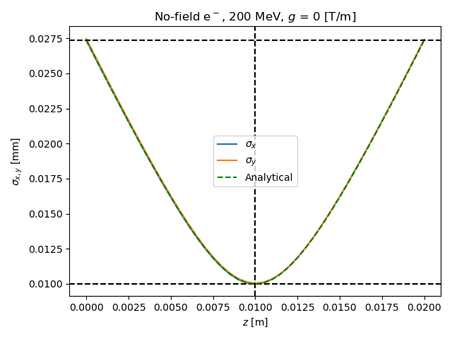
plot_APL_zero.py and output figures:
#!/usr/bin/env python3
#
# Copyright 2022-2025 ImpactX contributors
# Authors: Axel Huebl, Chad Mitchell, Kyrre Sjobak
# License: BSD-3-Clause-LBNL
#
# -*- coding: utf-8 -*-

import argparse

from analysis_APL import read_time_series
from plot_APL import millimeter, plot_sigmas, plt
from run_APL import analytic_sigma_function

# options to run this script, this one is used by the CTest harness
parser = argparse.ArgumentParser(
    description="Plot the ChrPlasmaLens_zero and ConstF_tracking_zero benchmarks."
)
parser.add_argument(
    "--save-png", action="store_true", help="non-interactive run: save to PNGs"
)
args = parser.parse_args()

# read reduced diagnostics
rbc = read_time_series("diags/reduced_beam_characteristics.*")

# Plot beam transverse sizes
plot_sigmas(rbc)

# Analytical estimates
# Start/end
plt.axhline(2.737665020201518e-05 * millimeter, ls="--", color="k")
# mid
plt.axhline(10e-6 * millimeter, ls="--", color="k")
plt.axvline(10e-3, ls="--", color="k")
# As function of s
(s, sigma) = analytic_sigma_function(0.0, 10e-6)
plt.plot(s, sigma * millimeter, ls="--", color="green", label="Analytical")

plt.legend(loc="center")
plt.title(r"No-field e$^-$, 200 MeV, $g$ = 0 [T/m]")
plt.tight_layout()

if args.save_png:
    plt.savefig("APL_zero-sigma.png")
else:
    plt.show()
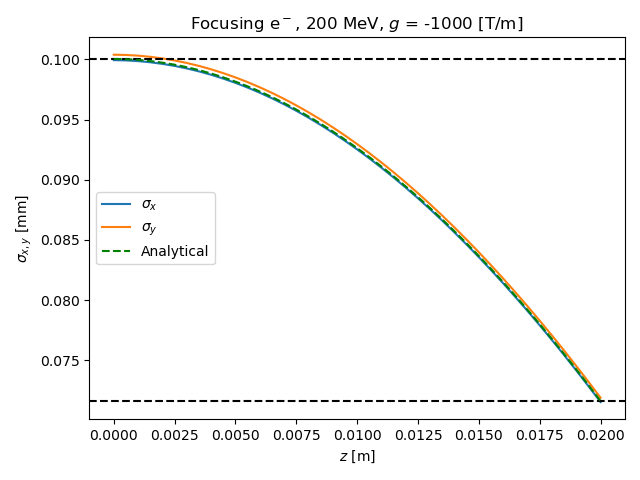
plot_APL_focusing.py and output figures:
#!/usr/bin/env python3
#
# Copyright 2022-2025 ImpactX contributors
# Authors: Axel Huebl, Chad Mitchell, Kyrre Sjobak
# License: BSD-3-Clause-LBNL
#
# -*- coding: utf-8 -*-

import argparse

from analysis_APL import read_time_series
from plot_APL import millimeter, plot_sigmas, plt
from run_APL import analytic_sigma_function

# options to run this script, this one is used by the CTest harness
parser = argparse.ArgumentParser(
    description="Plot the ChrPlasmaLens_focusing and ConstF_tracking_focusing benchmarks."
)
parser.add_argument(
    "--save-png", action="store_true", help="non-interactive run: save to PNGs"
)
args = parser.parse_args()

# import matplotlib.pyplot as plt

# read reduced diagnostics
rbc = read_time_series("diags/reduced_beam_characteristics.*")

# Plot beam transverse sizes
plot_sigmas(rbc)

# Analytical estimates
# Start/end
plt.axhline(7.161196476484095e-05 * millimeter, ls="--", color="k")
plt.axhline(100e-6 * millimeter, ls="--", color="k")
# plt.axvline(10e-3, ls="--", color="k")
# As function of s
(s, sigma) = analytic_sigma_function(-1000, 100e-6)
plt.plot(s, sigma * millimeter, ls="--", color="green", label="Analytical")

plt.legend(loc="center left")
plt.title(r"Focusing e$^-$, 200 MeV, $g$ = -1000 [T/m]")
plt.tight_layout()

if args.save_png:
    plt.savefig("APL_focusing-sigma.png")
else:
    plt.show()
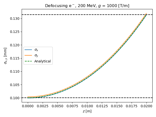
plot_APL_defocusing.py and output figures:
#!/usr/bin/env python3
#
# Copyright 2022-2025 ImpactX contributors
# Authors: Axel Huebl, Chad Mitchell, Kyrre Sjobak
# License: BSD-3-Clause-LBNL
#
# -*- coding: utf-8 -*-

import argparse

from analysis_APL import read_time_series
from plot_APL import millimeter, plot_sigmas, plt
from run_APL import analytic_sigma_function

# options to run this script, this one is used by the CTest harness
parser = argparse.ArgumentParser(
    description="Plot the ChrPlasmaLens_focusing and ConstF_tracking_focusing benchmarks."
)
parser.add_argument(
    "--save-png", action="store_true", help="non-interactive run: save to PNGs"
)
args = parser.parse_args()

# import matplotlib.pyplot as plt

# read reduced diagnostics
rbc = read_time_series("diags/reduced_beam_characteristics.*")

# Plot beam transverse sizes
plot_sigmas(rbc)

# Analytical estimates
# Start/end
plt.axhline(0.0001314429025974998 * millimeter, ls="--", color="k")
plt.axhline(100e-6 * millimeter, ls="--", color="k")
# plt.axvline(10e-3, ls="--", color="k")
# As function of s
(s, sigma) = analytic_sigma_function(+1000, 100e-6)
plt.plot(s, sigma * millimeter, ls="--", color="green", label="Analytical")

plt.legend(loc="center left")
plt.title(r"Defocusing e$^-$, 200 MeV, $g$ = 1000 [T/m]")
plt.tight_layout()

if args.save_png:
    plt.savefig("APL_defocusing-sigma.png")
else:
    plt.show()
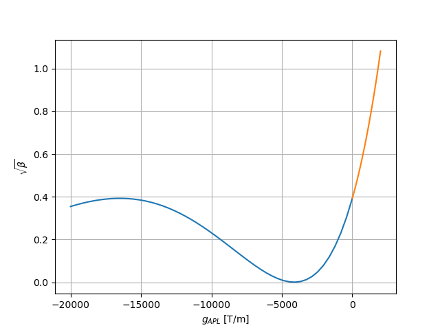
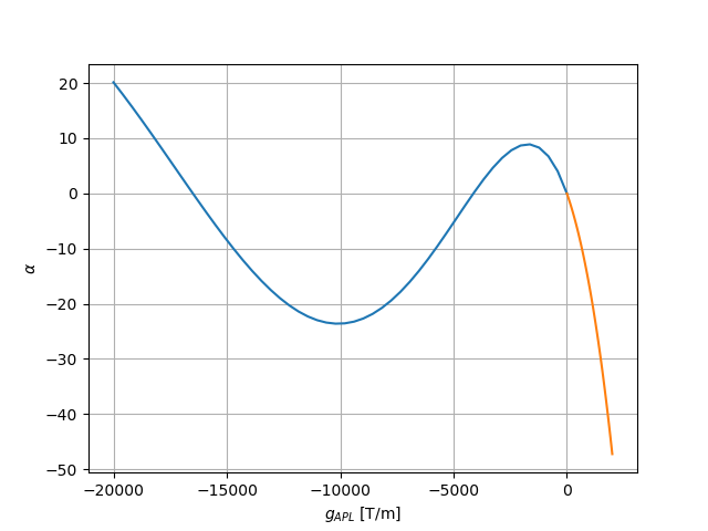
Additionally, it is also possible to run python3 plot_APL_analytical.py,
which plots the expected Twiss \(\alpha\) and \(\beta\) functions at the end of the lens
as a function of the lens gradient. This uses the stand-alone Twiss propagation function
analytic_final_estimate() from run_APL.py.
plot_APL_analytical.py and output figures:
#!/usr/bin/env python3
#
# Copyright 2022-2025 ImpactX contributors
# Authors: Axel Huebl, Chad Mitchell, Kyrre Sjobak
# License: BSD-3-Clause-LBNL
#
# -*- coding: utf-8 -*-

## Plots analytical Twiss parameters
#  as a function of APL gradient [T/m]

import argparse

import matplotlib.pyplot as plt
import numpy as np
from run_APL import analytic_final_estimate

# options to run this script, this one is used by the CTest harness
parser = argparse.ArgumentParser(
    description="Plot the ChrPlasmaLens_focusing and ConstF_tracking_focusing benchmarks."
)
parser.add_argument(
    "--save-png", action="store_true", help="non-interactive run: save to PNGs"
)
args = parser.parse_args()

rigidity_Tm = -0.6688305274603505  # [T*m], 200MeV electrons
APL_length = 20e-3  # [m]

# From "zero" test, sigma_mid = 10 um
# beta_0 = 0.029408806267344052 #[m]
# alpha_0 = 2.5484916642663316  #[-]
# From focusing, sigma_mid = 100 um
beta_0 = 0.39264381163450024
alpha_0 = 0.025484916642663318

# negative g (focusing, rigidity is also negative)
beta = []
alpha = []
g_def = np.linspace(0, -20000)
for APL_g in g_def:
    (beta_end, alpha_end, gamma_end) = analytic_final_estimate(
        APL_g, rigidity_Tm, APL_length, beta_0, alpha_0
    )

    beta.append(beta_end)
    alpha.append(alpha_end)

plt.figure(1)
plt.plot(g_def, beta)

plt.figure(2)
plt.plot(g_def, alpha)

# positive g (defocusing, rigidity is negative)
beta = []
alpha = []
g_def = np.linspace(0, 2000)
for APL_g in g_def:
    (beta_end, alpha_end, gamma_end) = analytic_final_estimate(
        APL_g, rigidity_Tm, APL_length, beta_0, alpha_0
    )

    beta.append(beta_end)
    alpha.append(alpha_end)

plt.figure(1)
plt.plot(g_def, beta)
plt.xlabel(r"$g_{APL}$ [T/m]")
plt.ylabel(r"$\sqrt{\beta}$")
plt.grid()
if args.save_png:
    plt.savefig("APL_analytical_sqrtBeta.png")

plt.figure(2)
plt.plot(g_def, alpha)
plt.xlabel("$g_{APL}$ [T/m]")
plt.ylabel(r"$\alpha$")
plt.grid()
if args.save_png:
    plt.savefig("APL_analytical_alpha.png")
else:
    plt.show()