Soft-Edge Quadrupole
This is a modification of the test for a matched electron beam propagating through a stable FODO cell, in which the quadrupoles have been replaced with soft-edge quadrupole elements. The on-axis field profile in this example has been chosen to correspond to the hard-edge limit, so the two tests should coincide.
We use a 2 GeV electron beam with initial unnormalized rms emittance of 2 nm.
In this test, the initial and final values of \(\sigma_x\), \(\sigma_y\), \(\sigma_t\), \(\epsilon_x\), \(\epsilon_y\), and \(\epsilon_t\) must agree with nominal values.
Run
This example can be run either as:
Python script:
python3 run_quadrupole_softedge.pyorImpactX executable using an input file:
impactx input_quadrupole_softedge.in
For MPI-parallel runs, prefix these lines with mpiexec -n 4 ... or srun -n 4 ..., depending on the system.
#!/usr/bin/env python3
#
# Copyright 2022-2023 ImpactX contributors
# Authors: Axel Huebl, Chad Mitchell
# License: BSD-3-Clause-LBNL
#
# -*- coding: utf-8 -*-

from impactx import ImpactX, distribution, elements

sim = ImpactX()

# set numerical parameters and IO control
sim.space_charge = False
# sim.diagnostics = False  # benchmarking
sim.slice_step_diagnostics = True

# domain decomposition & space charge mesh
sim.init_grids()

# load a 2 GeV electron beam with an initial
# unnormalized rms emittance of 2 nm
kin_energy_MeV = 2.0e3  # reference energy
bunch_charge_C = 1.0e-9  # used with space charge
npart = 10000  # number of macro particles

#   reference particle
ref = sim.beam.ref
ref.set_species("electron").set_kin_energy_MeV(kin_energy_MeV)

#   particle bunch
distr = distribution.Waterbag(
    lambdaX=3.9984884770e-5,
    lambdaY=3.9984884770e-5,
    lambdaT=1.0e-3,
    lambdaPx=2.6623538760e-5,
    lambdaPy=2.6623538760e-5,
    lambdaPt=2.0e-3,
    muxpx=-0.846574929020762,
    muypy=0.846574929020762,
    mutpt=0.0,
)
sim.add_particles(bunch_charge_C, distr, npart)

# add beam diagnostics
monitor = elements.BeamMonitor("monitor", backend="h5")

# design the accelerator lattice
ns = 1  # number of slices per ds in the element

quad1 = elements.SoftQuadrupole(
    name="quad1",
    ds=1.0,
    gscale=1.0,
    cos_coefficients=[2],
    sin_coefficients=[0],
    mapsteps=400,
    nslice=ns,
)

quad2 = elements.SoftQuadrupole(
    name="quad2",
    ds=1.0,
    gscale=-1.0,
    cos_coefficients=[2],
    sin_coefficients=[0],
    mapsteps=200,
    nslice=ns,
)

drift1 = elements.Drift(name="drift1", ds=0.25, nslice=ns)
drift2 = elements.Drift(name="drift2", ds=0.5, nslice=ns)

# assign a fodo segment
sim.lattice.extend([monitor, drift1, quad1, drift2, quad2, drift1, monitor])

# run simulation
sim.track_particles()

# clean shutdown
sim.finalize()
###############################################################################
# Particle Beam(s)
###############################################################################
beam.npart = 10000
beam.units = static
beam.kin_energy = 2.0e3
beam.charge = 1.0e-9
beam.particle = electron
beam.distribution = waterbag
beam.lambdaX = 3.9984884770e-5
beam.lambdaY = beam.lambdaX
beam.lambdaT = 1.0e-3
beam.lambdaPx = 2.6623538760e-5
beam.lambdaPy = beam.lambdaPx
beam.lambdaPt = 2.0e-3
beam.muxpx = -0.846574929020762
beam.muypy = -beam.muxpx
beam.mutpt = 0.0


###############################################################################
# Beamline: lattice elements and segments
###############################################################################
lattice.elements = monitor drift1 quad1 drift2 quad2 drift1 monitor
lattice.nslice = 1

monitor.type = beam_monitor
monitor.backend = h5

drift1.type = drift
drift1.ds = 0.25

quad1.type = quadrupole_softedge
quad1.ds = 1.0
quad1.gscale = 1.0
quad1.cos_coefficients = 2.0
quad1.sin_coefficients = 0.0
quad1.mapsteps = 400

drift2.type = drift
drift2.ds = 0.5

quad2.type = quadrupole_softedge
quad2.ds = 1.0
quad2.gscale = -1.0
quad2.cos_coefficients = 2.0
quad2.sin_coefficients = 0.0
quad2.mapsteps = 400


###############################################################################
# Algorithms
###############################################################################
algo.space_charge = false


###############################################################################
# Diagnostics
###############################################################################
diag.slice_step_diagnostics = false
Analyze
We run the following script to analyze correctness:
Script analysis_quadrupole_softedge.py
examples/quadrupole_softedge/analysis_quadrupole_softedge.py.#!/usr/bin/env python3
#
# Copyright 2022-2023 ImpactX contributors
# Authors: Axel Huebl, Chad Mitchell
# License: BSD-3-Clause-LBNL
#
import numpy as np
import openpmd_api as io
from scipy.stats import moment
def get_moments(beam):
"""Calculate standard deviations of beam position & momenta
and emittance values
Returns
-------
sigx, sigy, sigt, emittance_x, emittance_y, emittance_t
"""
sigx = moment(beam["position_x"], moment=2) ** 0.5 # variance -> std dev.
sigpx = moment(beam["momentum_x"], moment=2) ** 0.5
sigy = moment(beam["position_y"], moment=2) ** 0.5
sigpy = moment(beam["momentum_y"], moment=2) ** 0.5
sigt = moment(beam["position_t"], moment=2) ** 0.5
sigpt = moment(beam["momentum_t"], moment=2) ** 0.5
epstrms = beam.cov(ddof=0)
emittance_x = (sigx**2 * sigpx**2 - epstrms["position_x"]["momentum_x"] ** 2) ** 0.5
emittance_y = (sigy**2 * sigpy**2 - epstrms["position_y"]["momentum_y"] ** 2) ** 0.5
emittance_t = (sigt**2 * sigpt**2 - epstrms["position_t"]["momentum_t"] ** 2) ** 0.5
return (sigx, sigy, sigt, emittance_x, emittance_y, emittance_t)
# initial/final beam
series = io.Series("diags/openPMD/monitor.h5", io.Access.read_only)
last_step = list(series.iterations)[-1]
initial = series.iterations[1].particles["beam"].to_df()
final = series.iterations[last_step].particles["beam"].to_df()
# compare number of particles
num_particles = 10000
assert num_particles == len(initial)
assert num_particles == len(final)
print("Initial Beam:")
sigx, sigy, sigt, emittance_x, emittance_y, emittance_t = get_moments(initial)
print(f" sigx={sigx:e} sigy={sigy:e} sigt={sigt:e}")
print(
f" emittance_x={emittance_x:e} emittance_y={emittance_y:e} emittance_t={emittance_t:e}"
)
atol = 0.0 # ignored
rtol = 2.2 * num_particles**-0.5 # from random sampling of a smooth distribution
print(f" rtol={rtol} (ignored: atol~={atol})")
assert np.allclose(
[sigx, sigy, sigt, emittance_x, emittance_y, emittance_t],
[
7.5451170454175073e-005,
7.5441588239210947e-005,
9.9775878164077539e-004,
1.9959540393751392e-009,
2.0175015289132990e-009,
2.0013820193294972e-006,
],
rtol=rtol,
atol=atol,
)
print("")
print("Final Beam:")
sigx, sigy, sigt, emittance_x, emittance_y, emittance_t = get_moments(final)
print(f" sigx={sigx:e} sigy={sigy:e} sigt={sigt:e}")
print(
f" emittance_x={emittance_x:e} emittance_y={emittance_y:e} emittance_t={emittance_t:e}"
)
atol = 0.0 # ignored
rtol = 2.2 * num_particles**-0.5 # from random sampling of a smooth distribution
print(f" rtol={rtol} (ignored: atol~={atol})")
assert np.allclose(
[sigx, sigy, sigt, emittance_x, emittance_y, emittance_t],
[
7.4790118496224206e-005,
7.5357525169680140e-005,
9.9775879288128088e-004,
1.9959539836392703e-009,
2.0175014668882125e-009,
2.0013820380883801e-006,
],
rtol=rtol,
atol=atol,
)
FODO Cell Using Soft-Edge Quadrupoles
This is a modification of the example above, in which the quadrupoles have been replaced by soft-edge quadrupoles with an adjustable magnetic gap parameter, which allows the user to tune the rate of fringe field decay near the magnetic edge. In the limit \(g\rightarrow 0\), this model approaches the model of an ideal (hard-edge) quadrupole.
The on-axis gradient of the quadrupoles is given by an analytical function, namely:
\(k(z)=\frac{k_0}{2}\left\{\tanh\left(\frac{z+z_0}{g}\right)-\tanh\left(\frac{z-z_0}{g}\right)\right\}\)
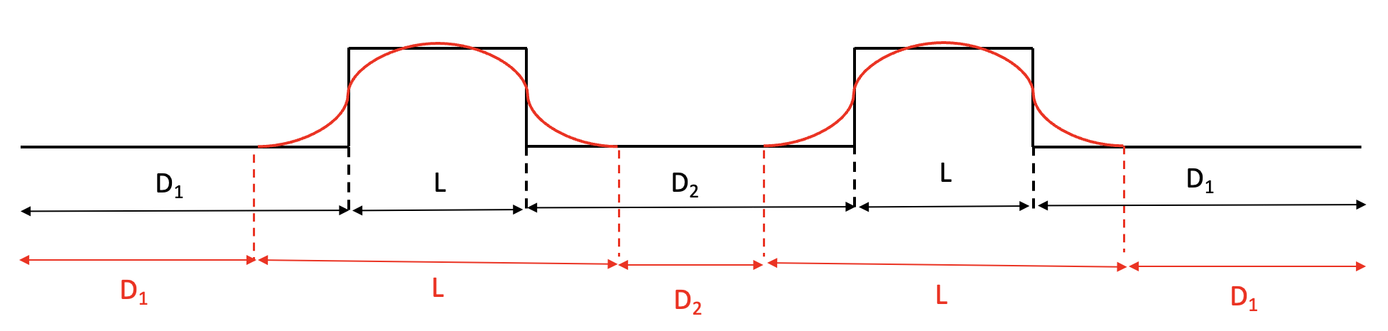
Fig. 5 Figure illustrating the layout of a FODO cell modeled using a hard edge (black) and soft-edge (red) quadrupole model. Curves approximately represent the magnitude of the on-axis quadrupole gradient.
The effect of the soft fringe field decay on the linear focusing is small but visible. In this test, the beam moments are compared against those used in the hard-edge limit.
The initial and final values of \(\sigma_x\), \(\sigma_y\), \(\sigma_t\), \(\epsilon_x\), \(\epsilon_y\), and \(\epsilon_t\) must agree with nominal values.
Run
This example can be run as:
Python script:
python3 run_fodo_softedge.py
For MPI-parallel runs, prefix these lines with mpiexec -n 4 ... or srun -n 4 ..., depending on the system.
#!/usr/bin/env python3
#
# Copyright 2022-2023 ImpactX contributors
# Authors: Axel Huebl, Chad Mitchell
# License: BSD-3-Clause-LBNL
#
# -*- coding: utf-8 -*-
import numpy as np
from impactx import ImpactX, distribution, elements
sim = ImpactX()
# set numerical parameters and IO control
sim.space_charge = False
# sim.diagnostics = False # benchmarking
sim.slice_step_diagnostics = True
# domain decomposition & space charge mesh
sim.init_grids()
# load a 2 GeV electron beam with an initial
# unnormalized rms emittance of 2 nm
kin_energy_MeV = 2.0e3 # reference energy
bunch_charge_C = 1.0e-9 # used with space charge
npart = 10000 # number of macro particles
# reference particle
ref = sim.beam.ref
ref.set_species("electron").set_kin_energy_MeV(kin_energy_MeV)
# particle bunch
distr = distribution.Waterbag(
lambdaX=3.9984884770e-5,
lambdaY=3.9984884770e-5,
lambdaT=1.0e-3,
lambdaPx=2.6623538760e-5,
lambdaPy=2.6623538760e-5,
lambdaPt=2.0e-3,
muxpx=-0.846574929020762,
muypy=0.846574929020762,
mutpt=0.0,
)
sim.add_particles(bunch_charge_C, distr, npart)
# add beam diagnostics
monitor = elements.BeamMonitor("monitor", backend="h5")
# design the accelerator lattice
ns = 10 # number of slices per ds in the element
# specify the on-axis field profile
zmin = -0.75 # lower value of on-axis longitudinal coordinate (in meters)
zmax = 0.75 # upper value of on-axis longitudinal coordinate (in meters)
nz = 401 # number of longitudinal sampling points to be used
g = 0.07 # gap parameter (in meters)
L_hardedge = 1.0 # length in the hard-edge limit
zdata = np.linspace(zmin, zmax, nz)
bdata = (
1.0
/ 2.0
* (
np.tanh((zdata + L_hardedge / 2.0) / g)
- np.tanh((zdata - L_hardedge / 2.0) / g)
)
)
# hard-edge lattice
quad1_he = elements.Quad(name="quad1", ds=1.0, k=1.0, nslice=ns)
quad2_he = elements.Quad(name="quad2", ds=1.0, k=-1.0, nslice=ns)
# design the accelerator lattice
quad1 = elements.SoftQuadrupole(
name="quad1",
ds=1.5,
gscale=1.0,
z=zdata,
gradient_on_axis=bdata,
ncoef=35,
mapsteps=200,
nslice=ns,
)
# design the accelerator lattice
quad2 = elements.SoftQuadrupole(
name="quad1",
ds=1.5,
gscale=-1.0,
z=zdata,
gradient_on_axis=bdata,
ncoef=35,
mapsteps=200,
nslice=ns,
)
# hard-edge lattice
drift1_he = elements.Drift(name="drift1", ds=0.25, nslice=ns)
drift2_he = elements.Drift(name="drift2", ds=0.5, nslice=ns)
# soft-edge lattice
drift1 = elements.Drift(name="drift1", ds=0.0, nslice=ns)
drift2 = elements.Drift(name="drift2", ds=0.0, nslice=ns)
# assign a fodo segment
sim.lattice.extend([monitor, drift1, quad1, drift2, quad2, drift1, monitor])
# sim.lattice.extend([monitor, drift1_he, quad1_he, drift2_he, quad2_he, drift1_he, monitor])
# run simulation
sim.track_particles()
# clean shutdown
sim.finalize()
Analyze
We run the following script to analyze correctness:
Script analysis_fodo_softedge.py
#!/usr/bin/env python3
#
# Copyright 2022-2023 ImpactX contributors
# Authors: Axel Huebl, Chad Mitchell
# License: BSD-3-Clause-LBNL
#

import numpy as np
import openpmd_api as io
from scipy.stats import moment


def get_moments(beam):
    """Calculate standard deviations of beam position & momenta
    and emittance values

    Returns
    -------
    sigx, sigy, sigt, emittance_x, emittance_y, emittance_t
    """
    sigx = moment(beam["position_x"], moment=2) ** 0.5  # variance -> std dev.
    sigpx = moment(beam["momentum_x"], moment=2) ** 0.5
    sigy = moment(beam["position_y"], moment=2) ** 0.5
    sigpy = moment(beam["momentum_y"], moment=2) ** 0.5
    sigt = moment(beam["position_t"], moment=2) ** 0.5
    sigpt = moment(beam["momentum_t"], moment=2) ** 0.5

    epstrms = beam.cov(ddof=0)
    emittance_x = (sigx**2 * sigpx**2 - epstrms["position_x"]["momentum_x"] ** 2) ** 0.5
    emittance_y = (sigy**2 * sigpy**2 - epstrms["position_y"]["momentum_y"] ** 2) ** 0.5
    emittance_t = (sigt**2 * sigpt**2 - epstrms["position_t"]["momentum_t"] ** 2) ** 0.5

    return (sigx, sigy, sigt, emittance_x, emittance_y, emittance_t)


# initial/final beam
series = io.Series("diags/openPMD/monitor.h5", io.Access.read_only)
last_step = list(series.iterations)[-1]
initial = series.iterations[1].particles["beam"].to_df()
final = series.iterations[last_step].particles["beam"].to_df()

# compare number of particles
num_particles = 10000
assert num_particles == len(initial)
assert num_particles == len(final)

print("Initial Beam:")
sigx, sigy, sigt, emittance_x, emittance_y, emittance_t = get_moments(initial)
print(f"  sigx={sigx:e} sigy={sigy:e} sigt={sigt:e}")
print(
    f"  emittance_x={emittance_x:e} emittance_y={emittance_y:e} emittance_t={emittance_t:e}"
)

atol = 0.0  # ignored
rtol = 2.2 * num_particles**-0.5  # from random sampling of a smooth distribution
print(f"  rtol={rtol} (ignored: atol~={atol})")

assert np.allclose(
    [sigx, sigy, sigt, emittance_x, emittance_y, emittance_t],
    [
        7.5451170454175073e-005,
        7.5441588239210947e-005,
        9.9775878164077539e-004,
        1.9959540393751392e-009,
        2.0175015289132990e-009,
        2.0013820193294972e-006,
    ],
    rtol=rtol,
    atol=atol,
)


print("")
print("Final Beam:")
sigx, sigy, sigt, emittance_x, emittance_y, emittance_t = get_moments(final)
print(f"  sigx={sigx:e} sigy={sigy:e} sigt={sigt:e}")
print(
    f"  emittance_x={emittance_x:e} emittance_y={emittance_y:e} emittance_t={emittance_t:e}"
)

atol = 0.0  # ignored
rtol = 2.2 * num_particles**-0.5  # from random sampling of a smooth distribution
print(f"  rtol={rtol} (ignored: atol~={atol})")

assert np.allclose(
    [sigx, sigy, sigt, emittance_x, emittance_y, emittance_t],
    [
        7.4790118496224206e-005,
        7.5357525169680140e-005,
        9.9775879288128088e-004,
        1.9959539836392703e-009,
        2.0175014668882125e-009,
        2.0013820380883801e-006,
    ],
    rtol=rtol,
    atol=atol,
)